GnssLogger Android App

This tutorial walks through how to parse the files obtained from Google’s GNSSLogger Android App. Details for each data type can be found in Google’s gps-measurement-tools repository.

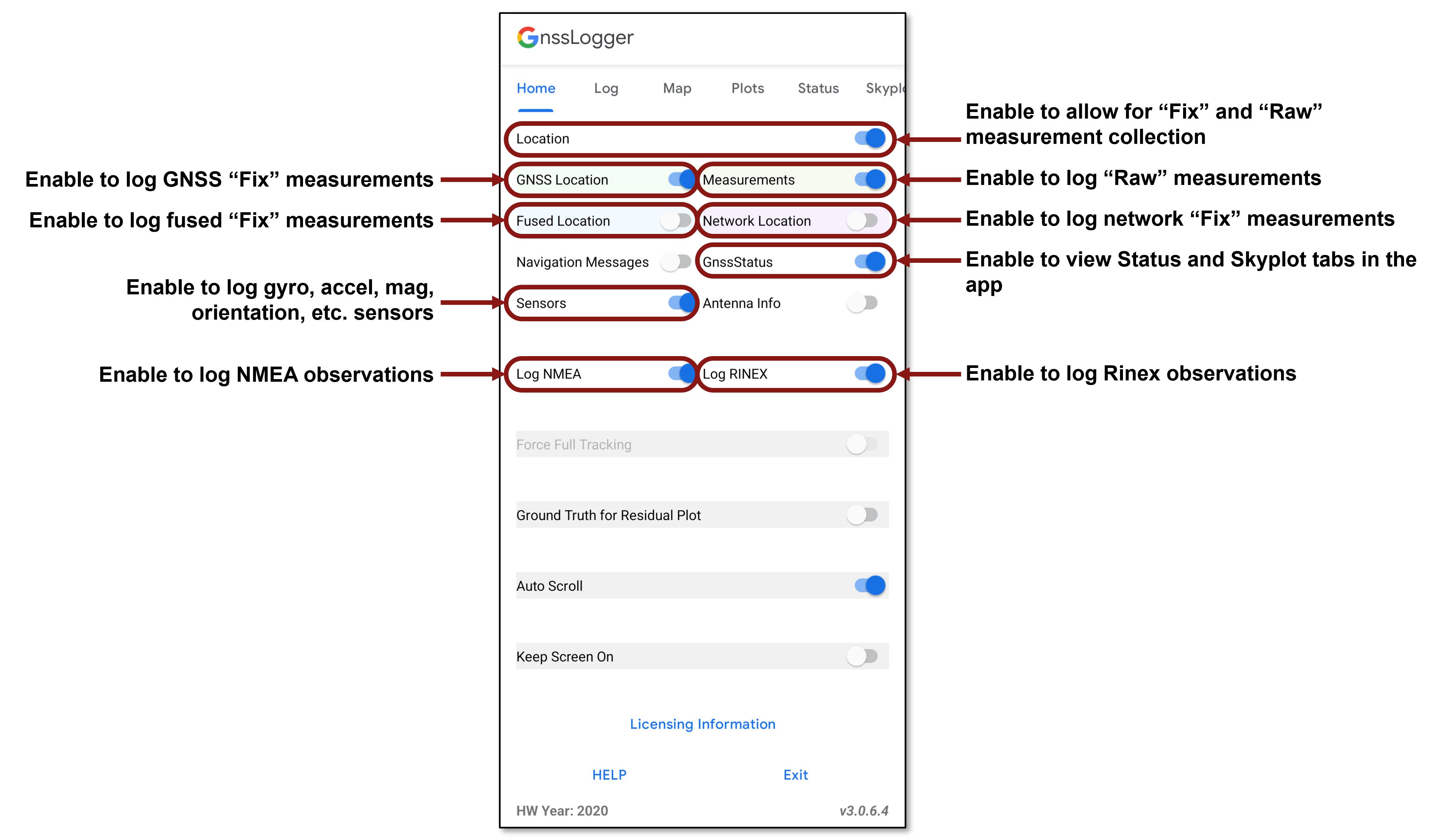
The toggle switches on the “Home” tab of the GNSSLogger app need to be set based on the type(s) of measurements you want to log: fixes, raw, NMEA, Rinex, sensors, etc.

After data is logged, the measurements can be saved immediately or retrieved at a later time within Android’s internal storage. Data can be found on the phone under a directory similar to: <phone>/Internal shared storage/Android/data/com.google.android.apps.location.gps.gnsslogger/files/gnss_log/

GnssLogger screenshot

Load gnss_lib_py into the Python workspace

[1]:

import numpy as np
import gnss_lib_py as glp
import matplotlib.pyplot as plt

Fix Measurements from gnss_log*.txt

The first type of measurements we can get is toggling a combination of “GNSS Location”, “Fused Location”, and/or “Network Location” in the GNSSLogger app. These location fixes are indicated with rows that start with “Fix” in the gnss_log.txt file output.

We start by downloading an example measurement file from the GNSSLogger Android App.

[2]:

glp.make_dir("../data")
!wget https://raw.githubusercontent.com/Stanford-NavLab/gnss_lib_py/main/data/unit_test/android/measurements/pixel6.txt --quiet -nc -O "../data/gnss_log.txt"

Load fix data into the existing glp.AndroidRawFixes class.

[3]:

fix_data = glp.AndroidRawFixes("../data/gnss_log.txt")

Based on the toggles you choose in the GNSSLogger app, you may have three different type of fixes: GNSS, network, and fused.

[4]:

fix_types = np.unique(fix_data["fix_provider"]).tolist()
fix_types

[4]:

['fused', 'gnss', 'network']

We will extract these three different type of fixes and rename their row names so that we can plot them as different colors all on the same map.

[5]:

fixes = []
for provider in fix_types:
    fix_provider = fix_data.where("fix_provider",provider)
    fix_provider.rename({"lat_rx_deg":"lat_rx_" + provider + "_deg",
                         "lon_rx_deg":"lon_rx_" + provider + "_deg",
                         "alt_rx_m":"alt_rx_" + provider + "_m",
                         }, inplace=True)
    fixes.append(fix_provider)

The GNSS, fused, and network location fixes are all shown in different colors in the map below.

[6]:

fig_fix = glp.plot_map(*fixes)
fig_fix.show()

Download example measurement file from the GNSSLogger Android App.

Raw Measurements from gnss_log*.txt

The secibd type of measurements we can get is by toggling “Measurements” in the GNSSLogger app. These are raw measurements indicated with rows that start with “Raw” in the gnss_log.txt file output.

We start by loading our previously downloaded raw data into the existing glp.AndroidRawGNSS class. When you load the data here, behind the scenes it will compute the raw pseudorange values optionally filter measurements based on a variety of conditions. See the the filter_raw_measurements reference documentation for details on the options for exisitng filter types.

[7]:

raw_data = glp.AndroidRawGnss(input_path="../data/gnss_log.txt",
                              filter_measurements=True,
                              measurement_filters={"sv_time_uncertainty" : 500.},
                              verbose=True)

sv_time_uncertainty removed 33

We now have many data fields with which to work. Details for each data field can be found in gnss_lib_py’s standard naming conventions or Google’s gps-measurement-tools repository.

[8]:

raw_data.rows

[8]:

['# Raw',
 'unix_millis',
 'TimeNanos',
 'LeapSecond',
 'TimeUncertaintyNanos',
 'FullBiasNanos',
 'BiasNanos',
 'BiasUncertaintyNanos',
 'DriftNanosPerSecond',
 'DriftUncertaintyNanosPerSecond',
 'HardwareClockDiscontinuityCount',
 'sv_id',
 'TimeOffsetNanos',
 'State',
 'ReceivedSvTimeNanos',
 'ReceivedSvTimeUncertaintyNanos',
 'cn0_dbhz',
 'PseudorangeRateMetersPerSecond',
 'PseudorangeRateUncertaintyMetersPerSecond',
 'AccumulatedDeltaRangeState',
 'accumulated_delta_range_m',
 'accumulated_delta_range_sigma_m',
 'CarrierFrequencyHz',
 'CarrierCycles',
 'CarrierPhase',
 'CarrierPhaseUncertainty',
 'MultipathIndicator',
 'SnrInDb',
 'gnss_id',
 'AgcDb',
 'BasebandCn0DbHz',
 'FullInterSignalBiasNanos',
 'FullInterSignalBiasUncertaintyNanos',
 'SatelliteInterSignalBiasNanos',
 'SatelliteInterSignalBiasUncertaintyNanos',
 'CodeType',
 'ChipsetElapsedRealtimeNanos',
 'signal_type',
 'gps_millis',
 'raw_pr_m',
 'raw_pr_sigma_m']

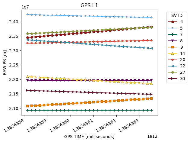
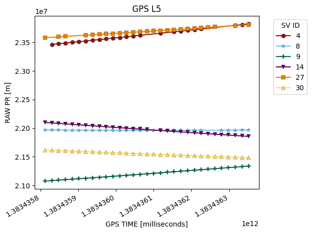
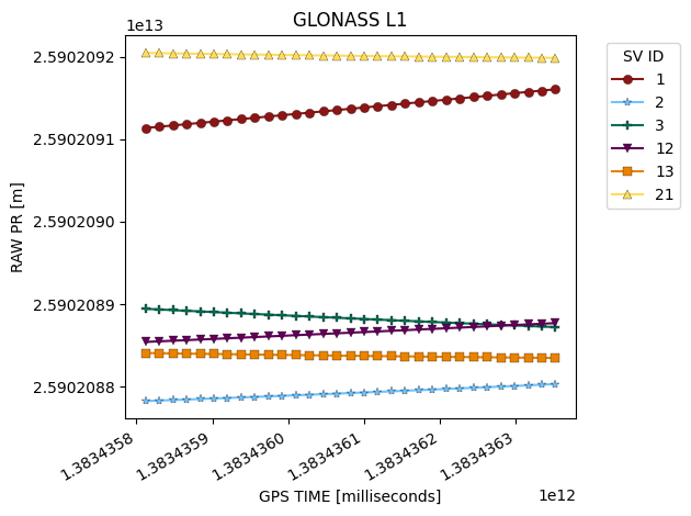
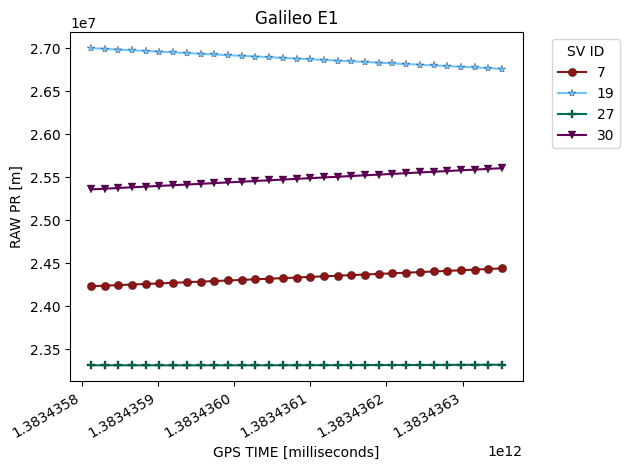
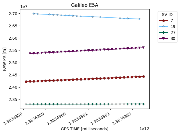
Let’s visualize the raw pseudoranges that have been compouted for us.

[9]:

figs = glp.plot_metric_by_constellation(raw_data,"gps_millis","raw_pr_m")

../../_images/tutorials_parsers_tutorials_android_notebook_23_0.png

../../_images/tutorials_parsers_tutorials_android_notebook_23_1.png

../../_images/tutorials_parsers_tutorials_android_notebook_23_2.png

../../_images/tutorials_parsers_tutorials_android_notebook_23_3.png

../../_images/tutorials_parsers_tutorials_android_notebook_23_4.png

Before we can compute a Weighted Least Squares position, we first need to add satellite positions to our data. This block may take a bit of time since it has to download ephemeris files from the internet. Turn on verbose=True to see the data sources it’s downloading.

[10]:

full_states = glp.add_sv_states(raw_data, source="precise", verbose=False)

We can then compute a “corrected” pseudorange by subtracting out each satellite’s respective clock bias.

[11]:

full_states["corr_pr_m"] = full_states["raw_pr_m"] \
                         + full_states['b_sv_m']

Since we haven’t yet computed any inter-constellation bias, we will crop down to only using GPS and Galileo measurements since the inter-constellation bias between them and GLONASS is quite large in this instance.

[12]:

full_states = full_states.where("gnss_id",("gps","galileo"))

We can now calculate our Weighted Least Squares position estimate.

[13]:

wls_estimate = glp.solve_wls(full_states)

Finally we’ll plot our state estimate on a map.

[14]:

raw_fig = glp.plot_map(wls_estimate)
raw_fig.show()

NMEA from gnss_log*.nmea

The third type of data that we can get from the GNSSLogger App is if “Log NMEA” is toggled. The NMEA data gives us a latitude and longitude directly.

We start by downloading an example NMEA log.

[15]:

glp.make_dir("../data")
!wget https://raw.githubusercontent.com/Stanford-NavLab/gnss_lib_py/main/data/unit_test/android/nmea/pixel6.nmea --quiet -nc -O "../data/gnss_log.nmea"

Load the NMEA data into the existing glp.Nmea class.

[16]:

nmea_data = glp.Nmea("../data/gnss_log.nmea")

We can plot the NMEA data on a map.

[17]:

nmea_fig = glp.plot_map(nmea_data)
nmea_fig.show()

We also have a few other fields explore.

[18]:

nmea_data.rows

[18]:

['lat_rx_deg',
 'lon_rx_deg',
 'gps_qual',
 'num_sats',
 'horizontal_dil',
 'alt_rx_m',
 'altitude_units',
 'geo_sep',
 'geo_sep_units',
 'age_gps_data',
 'ref_station_id',
 'status',
 'vx_rx_mps',
 'heading_raw_rx_deg',
 'gps_millis',
 'heading_rx_rad']

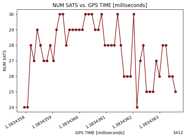
For example, we can plot the number of satellites over time.

[19]:

fig = glp.plot_metric(nmea_data,"gps_millis","num_sats")

../../_images/tutorials_parsers_tutorials_android_notebook_44_0.png

Rinex Observations

The last type of GNSS log that we can obtain from the GNSSLogger app is Rinex observations. We can obtain this data from certain phones if the “Log RINEX” option is toggled in the GNSSLogger app.

We start by downloading an example rinex observation log.

[20]:

glp.make_dir("../data")
!wget https://raw.githubusercontent.com/Stanford-NavLab/gnss_lib_py/main/data/unit_test/android/rinex_obs/pixel6.23o --quiet -nc -O "../data/gnss_log.23o"

Load the NMEA data into the existing glp.RinexObs class.

[21]:

rinex_data = glp.RinexObs("../data/gnss_log.23o")

One small pecularity about rinex observations logged with the GNSSLogger app is that their timestamps don’t account for the leapseconds since the start of the GPS epoch. Don’t worry though, with gnss_lib_py that’s a quick fix we can make.

[22]:

rinex_data["gps_millis"] -= glp.get_leap_seconds(rinex_data["gps_millis",0]) * 1E3

Before we can compute a Weighted Least Squares position, we first need to add satellite positions to our data. This block may take a bit of time since it has to download ephemeris files from the internet. Turn on verbose=True to see the data sources it’s downloading.

[23]:

full_states = glp.add_sv_states(rinex_data, source="precise", verbose=False)

We can then compute a “corrected” pseudorange by subtracting out each satellite’s respective clock bias.

[24]:

full_states["corr_pr_m"] = full_states["raw_pr_m"] \
                         + full_states['b_sv_m']

Since we haven’t yet computed any inter-constellation bias, we will crop down to only using GPS and Galileo measurements since the inter-constellation bias between them and GLONASS is quite large in this instance.

[25]:

full_states = full_states.where("gnss_id",("gps","galileo"))

We can now calculate our Weighted Least Squares position estimate.

[26]:

wls_estimate = glp.solve_wls(full_states)

Finally we’ll plot our state estimate on a map.

[27]:

raw_fig = glp.plot_map(wls_estimate)
raw_fig.show()

Sensor Measurements gnss_log*.txt

If the “sensors” option is toggled in the GNSSLogger app, then the gnss_log*.txt log file will contain a number of sensor measurements that can be extracted with built in Python classes.

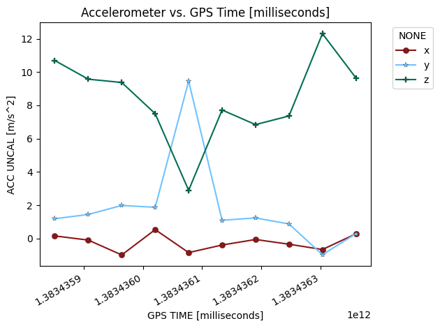
Accelerometer Measurements from gnss_log*.txt

[28]:

raw_data = glp.AndroidRawAccel(input_path="../data/gnss_log.txt")

[29]:

fig = glp.plot_metric(raw_data, "gps_millis","acc_x_uncal_mps2",label="x")
fig = glp.plot_metric(raw_data, "gps_millis","acc_y_uncal_mps2",label="y",fig=fig)
fig = glp.plot_metric(raw_data, "gps_millis","acc_z_uncal_mps2",label="z",fig=fig,
                     title="Accelerometer vs. GPS Time [milliseconds]")
ylabel = plt.ylabel("ACC UNCAL [m/s^2]")

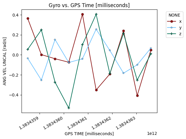
../../_images/tutorials_parsers_tutorials_android_notebook_66_0.png

Gyro Measurements from gnss_log*.txt

[30]:

raw_data = glp.AndroidRawGyro(input_path="../data/gnss_log.txt")

[31]:

fig = glp.plot_metric(raw_data, "gps_millis","ang_vel_x_uncal_radps",label="x")
fig = glp.plot_metric(raw_data, "gps_millis","ang_vel_y_uncal_radps",label="y",fig=fig)
fig = glp.plot_metric(raw_data, "gps_millis","ang_vel_z_uncal_radps",label="z",fig=fig,
                      title="Gyro vs. GPS Time [milliseconds]")
ylabel = plt.ylabel("ANG VEL UNCAL [rad/s]")

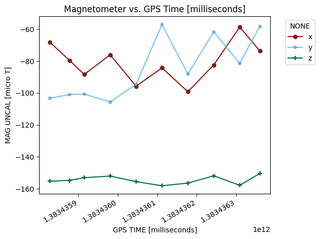
../../_images/tutorials_parsers_tutorials_android_notebook_69_0.png

Magnetometer Measurements from gnss_log*.txt

[32]:

raw_data = glp.AndroidRawMag(input_path="../data/gnss_log.txt")

[33]:

fig = glp.plot_metric(raw_data, "gps_millis","mag_x_uncal_microt",label="x")
fig = glp.plot_metric(raw_data, "gps_millis","mag_y_uncal_microt",label="y",fig=fig)
fig = glp.plot_metric(raw_data, "gps_millis","mag_z_uncal_microt",label="z",fig=fig,
                      title="Magnetometer vs. GPS Time [milliseconds]")
ylabel = plt.ylabel("MAG UNCAL [micro T]")

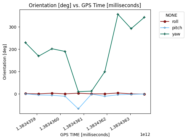
../../_images/tutorials_parsers_tutorials_android_notebook_72_0.png

Orientation Measurements from gnss_log*.txt

[34]:

raw_data = glp.AndroidRawOrientation(input_path="../data/gnss_log.txt")

[35]:

fig = glp.plot_metric(raw_data, "gps_millis","roll_rx_deg",label="roll")
fig = glp.plot_metric(raw_data, "gps_millis","pitch_rx_deg",label="pitch",fig=fig)
fig = glp.plot_metric(raw_data, "gps_millis","yaw_rx_deg",label="yaw",fig=fig,
                      title="Orientation [deg] vs. GPS Time [milliseconds]")
ylabel = plt.ylabel("Orientation [deg]")

../../_images/tutorials_parsers_tutorials_android_notebook_75_0.png